Distributions
Synthetic data involves a natural balance between data quality and privacy protection. Datasets that more closely reflect the original data may offer greater analytical value, while also requiring careful consideration of privacy risks. As a result, not every data quality metric will (or should) match perfectly.
Column distributions help you evaluate synthetic dataset quality, by comparing the similarity of real and synthetic columns. For Distributions, what counts as “good” value depends on your use case. Prioritize evaluating and improving statistical patterns that matter for your analysis, rather than optimizing all columns. For example, the distribution of an Age column might be more important than the Weather column in a prediction task for healthcare utilization. Find out more about how to improve the quality of the data generated here.
Column distributions are evaluated from two perspectives:
Overall Distribution: Compares all column distributions at once to determine the overall quality of the synthetic dataset.
Individual Column Distributions: Compares real and synthetic distributions for each column, to determine the quality of the synthetic column.
Overall Distribution
The “good” value depends on your use case. Synthetic data will never be a perfect replica, so focus on what matters most. For columns or use cases (e.g. data augmentation for machine learning) where retention of statistical attributes is important, you may require higher scores; if not lower scores may be acceptable.

Overall distribution compares all column distributions at once to determine the overall quality of the synthetic dataset.
You can assess the overall distribution of the synthetic dataset with the following metrics:
1. Multivariate Distribution Similarity
- Measures the overall distributional similarity between real and synthetic data across all columns at once. Higher values indicate better preservation of joint, multi-column patterns.
- Example: in the real data, older patients tend to have more hospital visits and higher treatment costs. A high multivariate similarity score means that this pattern across age, visits and cost together still appears in the synthetic data.
-
Find out more about metric used
Metric: Inverse Wasserstein distance.
Larger inverse Wasserstein Distance values mean that less computational effort is needed to transform the synthetic dataset distributions to resemble the real dataset.
Hence, higher values indicate better preservation of joint multi-column patterns, and the relationships between columns remain intact.
- Find out more about the difference between Multivariate Distribution Similarity and Overall Correlation (under "Relationships")
In summary, Multivariate Distribution Similarity checks realistic combinations, Overall Correlation checks relationships. You need both to assess synthetic data quality.
Multivariate Distribution Similarity
- Does the overall shape of the data as a whole look the same? This measures how similar the overall multi-column patterns in the synthetic data are compared to the real data, considering all columns together rather than pair by pair.
- Example: A low score may indicate records that look unrealistic as a whole, such as a 20-year-old patient with very high treatment costs and many hospital visits. These are values that may be possible individually but rarely occur together in the real data.
Overall Correlation (Associations Similarity) (Find out more)
- Are the relationships between columns preserved? This is a combined summary of all the column relationships.
- For example, if older patients in the real data generally have higher treatment costs, a low correlation score would indicate that this trend is weakened or missing, even if individual records still look plausible.
2. Overall Diversity
- Measures the variety and uniqueness of values across the entire synthetic dataset. Higher diversity indicates the synthetic data captures a wide range of patterns from the real data.
- Example: if the real dataset includes many different ages, diagnoses, and income ranges, a high diversity score means the synthetic data also contains a broad mix, rather than repeating the same few values.
-
Find out more about the metric used
A composite metric, calculated by multiplying three components:
- Variety (Uniqueness penalty): Geometric mean of % of unique values across columns.
Does the synthetic data have the same number of unique values as the real data?
Higher values indicate that the synthetic data contains as many unique values as the real data, and does not only contain a few unique values. - Spread (Entropy): Average normalised entropy across columns.
Do all values in the synthetic data appear with the frequency as the real data?
Higher values indicate that the synthetic data closely replicates the frequency of values in the real data, and does not cluster around a few values. - Detail Preservation: Average ratio of within-cluster variance over total variance across columns.
Do all values in the synthetic data appear with the frequency across groups as the real data?
Higher values indicate that the synthetic data closely replicates the frequency of data across groups as real data, and does not only cluster around a few values for some groups.
- Variety (Uniqueness penalty): Geometric mean of % of unique values across columns.
-
Find out more about reasons for poor diversity metric values
Example: Potential causes for poor overall diversity metric values
A poor overall diversity metric could be due to the following reasons:
- Variety (Uniqueness penalty): Numerical columns only contain a few unique values.
- Spread (Entropy): Categorical, numerical and datetime column values cluster around a few values.
- Detail preservation: Numerical column values only cluster around a few values for some groups.
In the following example, Mirage generates synthetic datasets that would have a poor overall diversity metric value from a real dataset with the following properties:
- Group A: Score values are mostly between 90-100, with the exception of one row.
- Group B: Score values are between 50-60.
Overall diversity component Real and synthetic datasets Explanation Variety (Uniqueness penalty) 
Numerical column "Score" only has two unique values in the synthetic dataset, which is less than the number of unique values in the real dataset (2 < 6). Spread (Entropy) 
- Synthetic categorical column "Group" only contains "A", and is missing the "B" category.
-
Synthetic numerical column "Score" has values clustered around a few values:
- Values are clustered between 95-96, instead of between 90-100.
- Values are clustered between 55-55.5, instead of between 50-60.
Detail preservation 
Synthetic numerical column "Score" only has values between 90-100 for Group A, and does not represent the outlier point in Group A that has a value between 50-60.
Individual Column Distributions

Individual column distributions compare each column in the synthetic dataset with the same column in the real dataset, to check how closely the synthetic values resemble the real ones.
You can assess each synthetic column with the following metrics:
- Univariate Distribution Similarity
- Measures the distributional similarity between a real column and its synthetic version, focusing on the pattern of values within that single column (e.g., ranges and frequencies). Higher values indicate better preservation of the column's individual distribution.
- Example: in the real data, most patients are aged 40–70, with fewer patients in their 20s or 80s. A high univariate similarity score means the synthetic "Age" column shows a similar pattern.
- Column-Level Diversity
- Measures the variety and uniqueness of values in a single column, comparing between the real and synthetic dataset. Higher values indicate that the synthetic column captures a wide range of patterns from the real column. The synthetic data captures rare and unique patterns, and does not just capture the most common patterns.
- Example: in the real data, most patients have 1 to 2 hospital visits, but a small number have 10 or more visits. A high diversity score means the synthetic "Number of Visits" column includes both the common cases and these rarer high-visit patients, instead of only repeating the most typical values.
- Domain Coverage
- Measures whether your synthetic column includes all possible values from your original data. Higher values indicate that your synthetic column represents the full range of your original data.
- Example: if the real "Diagnosis" column includes values like Diabetes, Hypertension, and Asthma, a high domain coverage score means all of these diagnoses also appear in the synthetic data; none are missing.
- Domain Adherence
- Domain adherence measures whether your synthetic column stays within the boundaries of your original data. Higher values indicate that the synthetic column does not create new, unexpected values.
- Example: if all patients in the real data are aged 0–100, a high domain adherence score means the synthetic "Age" column does not contain values like –5 or 130.
Data Provided By Column Type
| Column data type | Example |
|---|---|
| Categorical | 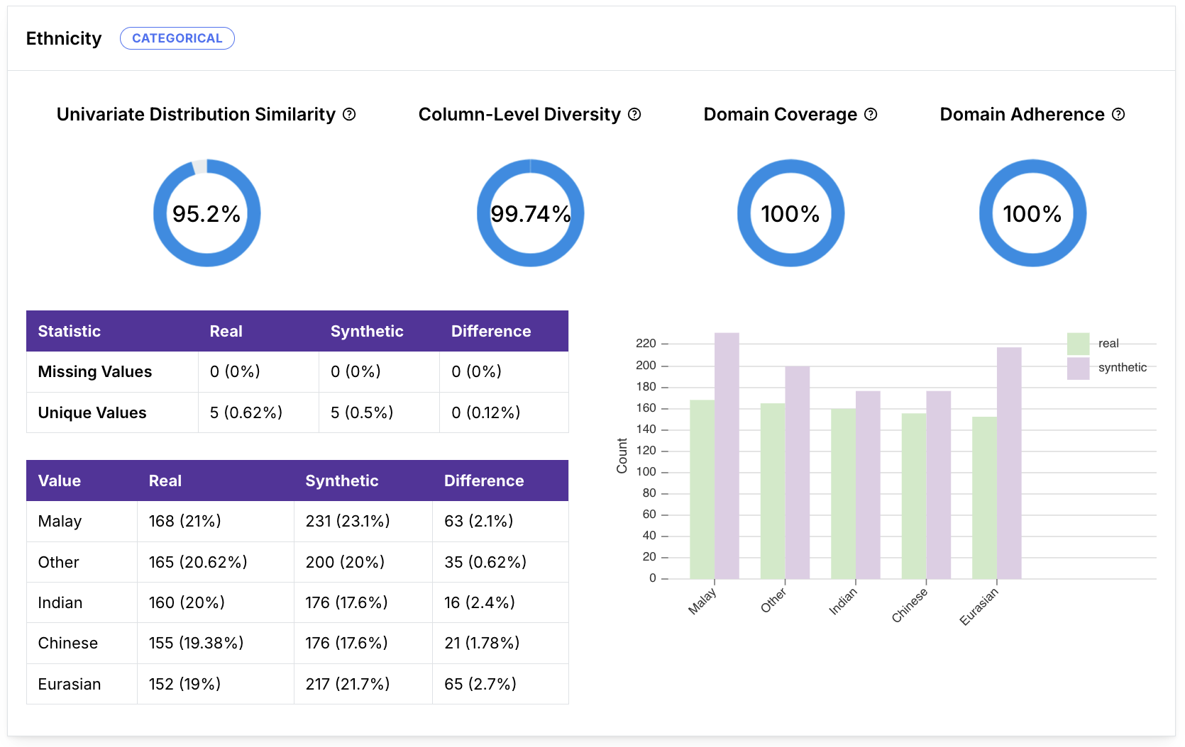 |
| Numerical | 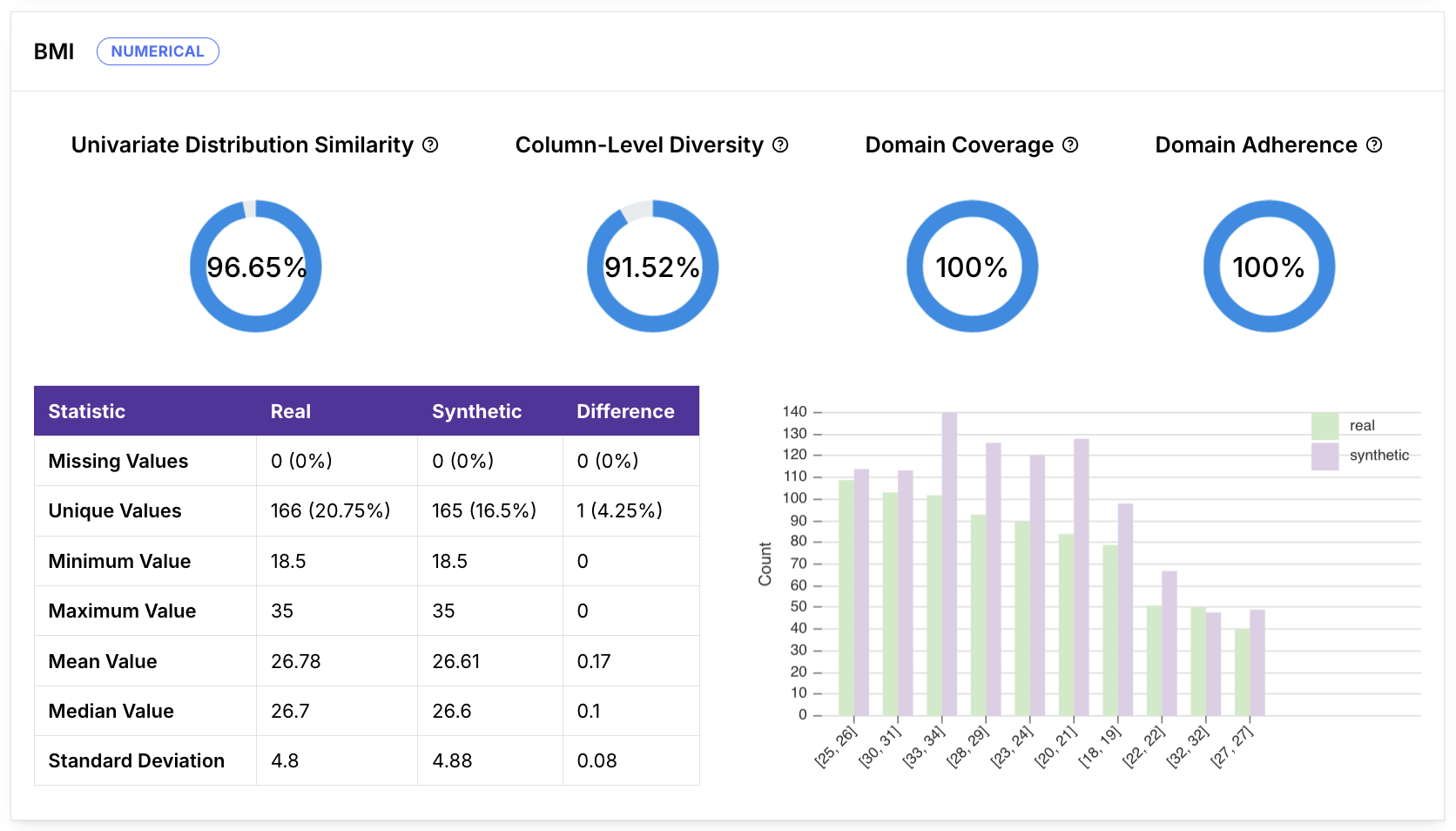 |
| Datetime | 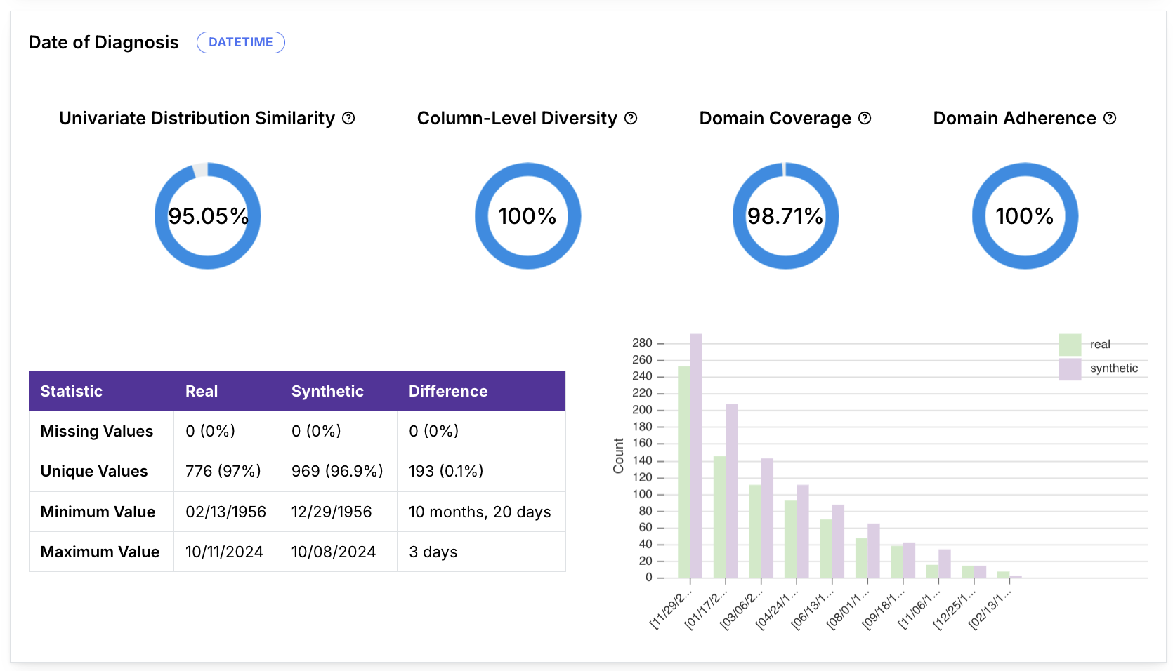 |
Example: Calculation of selected individual column distribution metrics
In the following example, Mirage generates a synthetic categorical column from a real categorical column.
The columns contain the following categories:
| Column | Categories |
|---|---|
| Real column | A, B |
| Synthetic column | A, B, C |

| Metric | Value | Rationale |
|---|---|---|
| Distribution similarity | 90% | Difference = % of values in Real data – % of values in Synthetic data
Distribution similarity = 100% - 0.5*20% (difference multiplied by 2) = 90% |
| Domain coverage | 100% | All categories in the real column (A and B) appear in the synthetic column at least once. |
| Domain adherence | 90% | Only 90% of the values in the synthetic column (A and B) appear in the original column, and the remaining 10% is an unexpected category (C). |
Sources:
Distribution similarity metrics (SDMetrics): TVComplement (categorical), KSComplement (numerical, datetime)
Domain coverage (SDMetrics): CategoryCoverage (categorical), RangeCoverage (numerical, datetime)
Domain adherence (SDMetrics): CategoryAdherence (categorical), BoundaryAdherence (numerical, datetime)